Under the Continuous Review Fixed Order Policy the Purchase Order Quantity
This chapter is from the book
Inventory Policy in a Fixed-Order Quantity System
A fixed-order quantity system is one of the most important in inventory management. For that reason we need to look at how to compute the two variables that define it: the order quantity Q and the reorder point ROP. Before we do that, however, we need to look at the assumptions this system makes. Most importantly, the system assumes that all the variables occur at a constant rate and their values are known with certainty. For example, the system assumes that the demand, D, occurs at a constant rate and that there is no variability in demand. Also, the lead time, L, is constant, the holding cost, H, is known and fixed, as are stockout cost, S, and unit price, C. Although these assumptions are not realistic the model is highly robust and provides excellent results despite these assumptions.
How Much to Order?
The first decision in the fixed-order quantity model is to select the order quantity Q. Recall that there are a number of inventory costs, most notably inventory holding cost and ordering cost. We want to select the "best" order quantity that minimizes these costs—the EOQ mentioned previously. This is computed by looking at the total annual inventory cost and finding the order quantity that minimizes it. Consider that the total annual cost is comprised of annual purchase cost, annual ordering cost, and annual holding cost, and looks as follows:
- Total cost = Purchase cost + Ordering cost + Holding cost
- TC = DC + (D/Q) S + (Q/2) H
where
- TC = Total cost
- D = Annual demand
- C = Unit cost
- Q = Order quantity
- S = Ordering cost
- H = Holding cost
The first term in the equation, DC, is the annual purchase cost for items. It is comprised of annual demand (D) times the unit cost of each item (C). The second term (D/Q) S is the annual ordering cost. It is computed as the number of orders placed per year (D/Q), times the cost of each order, S. Finally, the third term is annual holding cost where (Q/2) is the average inventory held. Remember that our maximum inventory is Q units when the order is received. When inventory is depleted we have zero. Therefore on average we have Q/2 units in inventory. H is the annual holding cost per unit of inventory.
The behavior of the two costs is shown in Figure 1-7. Notice that inventory holding cost increases with the order quantity, Q. The reason is that higher order quantities mean holding more inventory. However, this also means that we are ordering less frequently so ordering cost decreases. The opposite is true as the order quantity Q is decreased. A smaller order quantity results in a lower holding cost, but a higher ordering cost, as we are ordering more frequently.
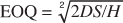
The objective is to pick an order quantity that minimizes the sum of both the holding and ordering costs, which is the minimum point on the total cost curve. To compute this we use calculus and end up with the following classic computation of the "best" or optimal order quantity, the EOQ:
When to Order?
The EOQ answers the question of how much to order, but we still need to determine when to order. Assume that the demand rate (D) and lead time (L) are constant and known with certainty. In that case the ROP would simply be enough inventory to ensure that demand is covered during the length of the lead time. In this simple case, the ROP would be computed as
- ROP = demand during lead time
- ROP = D L
Let's assume that lead time L for a product is one week and the demand, d, is 250 units per week. The ROP would be
- Reorder Point = ROP = D x L = 1 week x 250 = 250 units
This means that every time inventory reaches 250 units an order is placed for the economic order quantity Q.
Unfortunately, D and L are rarely fixed, and demand is often higher than expected. As a result we often have to carry a bit more inventory to address this uncertainty. This is called safety stock or buffer stock and is inventory we carry in addition to the demand during lead time. Safety stock is added to the ROP calculation and is computed as follows:
- ROP = demand during lead time + safety stock
- ROP = D L + SS
Safety stock is computed based on the service level a company wants to maintain, which is simply the chance that we will not run out of stock. This is set by the company based on the level of service it wants to provide for a particular product and customer base. Higher service levels mean higher levels of inventory. Another factor that is used to compute safety stock is the variability of demand. The higher the variability and the higher the service level the higher the safety stock, or the amount added to the final computation of the ROP.
Source: https://www.informit.com/articles/article.aspx?p=2167438&seqNum=8
0 Response to "Under the Continuous Review Fixed Order Policy the Purchase Order Quantity"
Post a Comment